Note: All comments and opinions expressed on this blog are mine alone and do not necessarily reflect those of my employers, past or present.
본 게시글의 원문은 Yann Debray의 MATLAB with Python Book 입니다. 해당 책은 MIT 라이센스를 따르기 때문에 개인적으로 번역하여 재배포 합니다. 본 포스팅에는 추후 유료 수익을 위한 광고가 부착될 수도 있습니다.
MIT License

Copyright (c) 2023 Yann Debray

Permission is hereby granted, free of charge, to any person obtaining a copy
of this software and associated documentation files (the "Software"), to deal
in the Software without restriction, including without limitation the rights
to use, copy, modify, merge, publish, distribute, sublicense, and/or sell
copies of the Software, and to permit persons to whom the Software is
furnished to do so, subject to the following conditions:

The above copyright notice and this permission notice shall be included in all
copies or substantial portions of the Software.

THE SOFTWARE IS PROVIDED "AS IS", WITHOUT WARRANTY OF ANY KIND, EXPRESS OR
IMPLIED, INCLUDING BUT NOT LIMITED TO THE WARRANTIES OF MERCHANTABILITY,
FITNESS FOR A PARTICULAR PURPOSE AND NONINFRINGEMENT. IN NO EVENT SHALL THE
AUTHORS OR COPYRIGHT HOLDERS BE LIABLE FOR ANY CLAIM, DAMAGES OR OTHER
LIABILITY, WHETHER IN AN ACTION OF CONTRACT, TORT OR OTHERWISE, ARISING FROM,
OUT OF OR IN CONNECTION WITH THE SOFTWARE OR THE USE OR OTHER DEALINGS IN THE
SOFTWARE.
본 게시물에서 활용된 소스 코드들은 모두 Yann Debray의 GitHub Repo에서 확인할 수 있습니다.
7.4. Simulink 모델을 배포를 위해 Python 패키지로 내보내기
네 번째 시나리오에서는 Simulink 모델을 Python 기반의 프로덕션 시스템에 배포하는 것이 목표입니다.
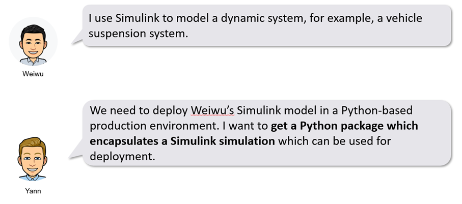
여기서의 단계는 동일합니다. 유일한 차이점은 모델을 배포용으로 구성해야 한다는 것입니다. 모든 Simulink 모델이 배포 가능한 것은 아니기 때문입니다. 따라서 시뮬레이션 입력 객체를 호출하기 전에 다음 줄을 추가하여 변환해야 합니다:
si = simulink.compiler.configureForDeployment(si);
그런 다음 다음 단계는 MATLAB 함수를 Python 패키지로 컴파일하는 것입니다:
appFile = which('sim_the_model2');
outDir = fullfile(origDir,'sim_the_model2_python_package_installer');
compiler.build.pythonPackage(appFile, ...
        'PackageName','sim_the_model2', ...
        'OutputDir',outDir);
마지막으로 Python 패키지를 설치하고 다음과 같이 호출해야 합니다:
import sim_the_model2
import matplotlib.pyplot as plt
# sim_the_model 패키지 초기화
mlr = sim_the_model2.initialize()
# 두 번의 sim_the_model 호출 결과를 저장할 res 리스트 할당
res = [0]*2
# 첫 번째 시뮬레이션: 기본 매개변수 값 사용: Mb = 1200 Kg
res[0] = mlr.sim_the_model2('StopTime', 30)
# 두 번째 시뮬레이션: 조정 가능한 매개변수에 대한 새로운 값 사용
tunableParams = {
'Mb': 5000.0 # 차체 질량 Kg에 대한 새로운 매개변수 사용
}
res[1] = mlr.sim_the_model2('StopTime', 30, 'TunableParameters', tunableParams)
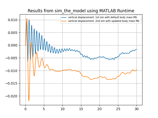
# 결과를 플로팅
cols = plt.rcParams['axes.prop_cycle'].by_key()['color']
fig, ax = plt.subplots(1, 1, sharex=True)
ax.plot(res[0]['vertical_disp']['Time'], res[0]['vertical_disp']['Data'], color=cols[0],
label="수직 변위: 기본 차체 질량 Mb로 첫 번째 시뮬레이션")
ax.plot(res[1]['vertical_disp']['Time'], res[1]['vertical_disp']['Data'],
color=cols[1], label="수직 변위: 업데이트된 차체 질량 Mb로 두 번째 시뮬레이션")
ax.grid()
lg = ax.legend(fontsize='x-small')
lg.set_draggable(True)
ax.set_title("MATLAB Runtime을 사용한 sim_the_model 결과")
plt.show()
mlr.terminate() # MATLAB Runtime 종료
이 코드는 다음과 같은 Python 플롯을 생성합니다: